Web page maintained by Evans M. Harrell, II, harrell@math.gatech.edu.
p(x,y) u_x + q(x,y) u_y + r(x,y) u = 0 (2.1)
and three ordinary differential equations:
A(F(dx,dt) = p(x,y),F(dy,dt) = q(x,y)) (2.2)
F(dz,dt) + s(t) z = 0 (2.3)
where s(t) is to be defined below.
To make the connection with the previous section and between (2.1) and (2.2), suppose that x(t) and y(t) are functions from [0,*) to the reals that satisfy the system of equations (2.2) with initial conditions:
F(dx,dt) = p(x,y), x(0) = 0
F(dy,dt) = q(x,y), y(0) = [[eta]].
These are equations such as those we solved in the last section. Suppose the functions p and q have the properties required in the previous section. Choose a point {a,b} in the region where the equations
x(t) = a
y(t) = b
can be solved for [[eta]] and t uniquely in terms of a and b. Geometrically, this locates the initial point {0,[[eta]]} on the y axis so that a point following along the trajectory given parametrically by the functions x and y and beginning at {0,[[eta]]} arrives at {a,b} in time t. This is a characteristic curve for (2.1) beginning at {0,[[eta]]}.
We derive the solution surface by thinking of the smooth surface u(x(t),y(t)) above the trajectories {x(t), y(t)}. Here's a way to describe its evolution there. We choose r from (2.1) and solve (2.3) for z where
s(t) = r(x(t), y(t)). (2.4)
Then define u implicitely:
u(x(t), y(t)) = z(t). (2.5)
It follows that
p(x,y) u_x + q(x,y) u_y + r(x,y) u
= x[[minute]] u_x + y[[minute]] u_y + r(x,y) u
(2.6)
= F(d ,dt)u(x(t),y(t)) + r(x(t),y(t)) u(x(t),y(t))
= F(dz,dt) + s(t) z = 0.
Because z(0) = u(x(0), y(0)) = u(0,[[eta]]), we know how the initial condition for [[eta]] should be made:
z(0) = u(0,[[eta]]).
The function z depends on t and [[eta]]. One could write z = z(t,[[eta]]).
(Some comments by Evans Harrell.)
Summary:
We have the recipe for providing a solution for (2.1):
(1)     Solve for the characteristics as in (2.2) with initial conditions.
(2)     Define s(t) from (2.4).
(3)     Solve (2.3) with initial conditions z(0) = u(0,[[eta]]).
(4)     Invert the equations x = x(t,[[eta]]) and y = y(t,[[eta]]) to solve
        for t and [[eta]] in terms of x and y:  t = t(x,y), [[eta]] =
        [[eta]](x,y).
(5)     Compose u(x,y) = z(t,[[eta]]) = z(t(x,y), [[eta]](x,y)).
Example 2.1:
We generate a solution to the partial differential equation
1 u_x + 2 u_y + 3 u = 0 (2.7)
with initial conditions
U(0,y) = exp(-y^2).
Following the procedure suggested above, we solve the system of ordinary differential equations
x[[minute]](t) = 1, x(0) = 0,
y[[minute]](t) = 2, y(0) = [[eta]].
This has an easy solution
x(t) = t and y(t) = 2t + [[eta]]. (2.8)
We must now solve the differential equation that arises from the context of the partial differential equation
F(dz,dt) + 3z = 0, z(0) = exp(-[[eta]]^2).
Of course, this has solution
z(t) = exp(-3t) exp(-[[eta]]^2). (2.9)
It remains to "invert" the relation (2.6) between {x,y} and {t,[[eta]]}. In fact,
[[eta]] = y- 2x
t = x. (2.10)
One should check now to see that substitution of (2.7) into (2.5) provides a solution for the differential equation. The substitution yields
u(x,y) = exp(-3x) exp(-[y-2x]^2). (2.11)
Here is a Maple verification that this answer is correct:
> u:=(x,y) -> exp(-3*x)*exp(-(y-2*x)^2);
> diff(u(x,y),x)+2*diff(u(x,y),y)+3*u(x,y);
> simplify(");
> u(0,y);
Because we now have the powerful mathematical and graphing tool Maple , we can not resist looking at the graph of this solution.
> plot3d(u(x,y),x=0..3,y=-3..3);
Figure 2.1: Graph of the solution for Example 2.1
It might help intution to look at the above graph and imagine the lines y = 2x + [[eta]] and to see how the initial distribution decays along those curves.
Summary for Example 2.1: The characteristics for
1 u_x + 2 u_y + 3 u = 0
are the lines x(t) = t, y(t) = 2 t + [[eta]]
or y = 2 x + [[eta]].
The determining differential equation along the characteristic is
F(dz,dt) + 3 z = 0, z(0) = exp(-3 [[eta]]^2)
which has solution exp(-3t) exp(- [[eta]]^2). After inverting the relationship between {x, y} and {t, [[eta]]}, we find the solution for the partial differential equation is
u(x,y) = exp(-3x) exp(-[y - 2x]^2).
Example 2.2:
We find solutions for the differential equation
u_x + y u_y + x u = 0 for -* < y < *, 0 < x (2.12)
subject to the initial condition
u(0,y) = sin(y).
We also draw graphs of the parameteric curves x(t,[[eta]]) and y(t,[[eta]]) and of the solution surface u(x,y).
The parameteric curves x and y are determined by the equations
F(dx,dt) = 1, with x(0) = 0,
F(dy,dt) = y, with y(0) = [[eta]].
This system of equations has solution
x(t,[[eta]]) = t,
y(t,[[eta]]) = [[eta]] exp(t).
We invert and find [[eta]] and t as functions of x and y:
t = x and [[eta]] = y exp(-x).
The determining differential equation for u that is associated with this system is
F(dz,dt) + t z = 0, with z(0) = sin([[eta]]).
This equation has solution
z(t) = exp(-t^2/2) sin([[eta]]).
Finally, we substitute the inversion to x and y coordinates:
u(x,y) = exp(-x^2/2) sin(y e^-x). (2.13)

Figure 2.2 a. Characteristic Curves

Figure 2.2 b. Solution Surface
The Figure 2.2a has the characteristic curves drawn as trajectories {x(t),y(t)}. Figure 2.2b shows the graph of u. Again, it is of value to visualize in this three dimensional graph how the initial value decays and spreads along the trajectories {x,y}.
The trajectories {x(t),y(t)} are called the characteristics curves associated with the partial differential equation. One speaks of solving the partial differential equation by the method of characteristics.
Surely there are interesting questions remaining here:
(1)     How robust is this method?
(2)     How bizarre might the characteristic curves be?
(3)     Since one curve carries information from the initial value, what
        happens if a curve from a point [[eta]] where the initial data was
        small gets close to a curve from another point [[eta]] where the data
        was large. (One might imagine riding gently along one characteristic
        curve and looking up to see a huge wave bearing down along another
        characteristic curve that started at some different initial value!)
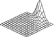
Example 2.3. "Surfer's Delight"
Let p(x,y) = 1 and
q(x,y) = BLC{(A(-y if y >= 0, 0 if y <= 0)).
Consider u that satisfies
p(x,y) u_x + q(x,y) u_y = 0, with u(0,y) = [[pi]]/2+ arctan(y). (2.14)
This equation has solution u(x,y) = [[pi]]/2+ arctan(y e^x) if y > 0. The graph of the solution suggests an approach to discontinuity of the solution for x large and |y| small.
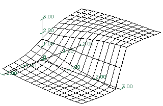
Figure 2.3. Graph of [[pi]]/2+ arctan(y e^x).
Summary for visualization
of
first order, quasilinear partial differential equations.
We will explain this summary with the example
x u_x - xy u_y = u for x > 1, u(1,y) = f(y) for all y.
For the purpose of analyzing this problem, it makes the calculus easier to change the equation to
u_x - y u_y = u/x for x > 1.
Visualization of the characteristics.
There are two methods to use Maple to visualize the characteristics.
(1) Use the numerical integration procedures, or
(2) solve for the characteristic curves analytically and graph the solutions.
Implementation of Method 1:
This method is more appropriate when the characteristics can not be found analytically.
> with(DEtools):
> eqns:=[diff(x(t),t)=1,diff(y(t),t)+ y(t)= 0];
inits:={[0,1,-2],[0,1,-1],[0,1,1],[0,1,2],[0,1,3]};
> phaseportrait(eqns,[x,y],0..2,inits,stepsize=0.1,x=-1/2..3,y=-1..3);
Implementation of method 2:
The characteristics solve the equations
x' = 1 with x(0) = 1 and y' = -x y with y(0) = eta.
These two equations can be solved with Maple .
> dsolve({diff(x(t),t)=1,diff(y(t),t)+ y(t)= 0, x(0)=1, y(0) = eta},
{x(t),y(t)});
> assign(");
Having the solutions, we draw their graphs.
> plot({[t+1,-2*exp(-t),t=0..2],[t+1,-1*exp(-t),t=0..2],
[t+1,1*exp(-t),t=0..2],[t+1,2*exp(-t),t=0..2],
[t+1,-1*exp(-t),t=0..2],[t+1,3*exp(-t),t=0..2]},
x=-1/2..3,y=-1..3);
Visualization of the solution surfaces.
There are three methods to use Maple to visualize the solution surfaces.
(1) Use the numerical integration procedures, or
(2) Graph the solutions parametrically, or
(3) Graph the solutions numerically.
Implementation of method 1:
This method uses the numerical procedures in Maple . It is more appropriate when the characteristics can not be found analytically.
> restart: with(DEtools);
> PDEplot([1,-y,-u/x],[x,y,u],[1,s,exp(-s^2)],s=-1..3,numchar=20,
axes=NORMAL, orientation = [-50,40]);
Implementation of Method 2.
This method plots the surface parametrically. It is more appropriate when the equations for the characteristics can not be inverted. First the characteristics are determined; as above,
x(t) = t+1 and y(t) = eta*exp(-t).
The function z(t) satisfies the differential equation
z'(t) = z(t)/x(t) = z(t)/(t+1), with z(0) = exp(-eta^2).
We solve this equation.
> dsolve({diff(z(t),t) = z(t)/(t+1),z(0) = exp(-eta^2)},z(t));
Instead of inverting the equations here, we plot {x(t),y(t),z(t)} parametrically.
> plot3d([t+1,eta*exp(-t),exp(-eta^2)*(t+1)],t=0..2,eta=-1..3,
axes=NORMAL, orientation = [-5,45]);
Implementation of Method 2.
This method plots the surface analytically. We must invert the characteristic equations.
> restart;solve({t+1=a,eta*exp(-t)=b},{t,eta});
> assign(");
> u:=(a,b)->exp(-eta^2)*(t+1);
> u(a,b);
> plot3d(u(a,b),a=1..3,b=-1..3,axes=NORMAL);
Exercises
(2.1) Solve these partial differential equations by the method of characteristics. Sketch the characteristics, and the solution's surface.
(a) u_x + u_y = 0, -* < y < *, 0 < x with u(0,y) = cos(y).
(b) 1u_x + yu_y + 2u = 0, -* < y < *, 0 < x with u(0,y) = sin(y).
(2.2) Solve these partial differential equations:
(a) x u_x +y u_y + x = 0, u(1,y) =y.
(b) u_x = 3x^2, u(0,y) = f(y).
(c) x u_x + y u_y = x y (x^2 + 1), u(1,y)=y.
(d) x^2 u_x + y^2 u_y = u, u(1,y) = y.
(2.3) Solve these partial differential equations:
(a) xu_x + yu_y = -5u, u(1,y) = sin(y).
(b) u_x + u_y + x u = 0, u(0,y) = f(y).
(c) u_x + 2 u_y +2 u = 0, u(x,x) = f(x). (Attention: the initial condition is on the line y = x.)
(d) x u_x + y u_y = u+1, u(x,x^2) = x^2.
(2.4) Solve these partial differential equations
(a) x u_x - y u_y = y, with u(1,y) = f(y)
(b) x u_x + y u_y = 2 u, with u(0,y) = f(y)
(c) x^2 u_x - y^2 u_y = y^2 - x^2 , with u(1,y) = f(y).
(2.5) Solve these partial differential equations
(a) u_x + u_y = 0, u(1,y) = cos(y)
(b) x^2 u_x + y^2 u_y - (x+y) u = 0, u(1,y) =exp(-y^2).
(2.6) Make four partial differential equations, each with initial value u(0,y) = exp(-y^2) and each having one of these properties:
a. the distribution moves along characteristics with slope 1 and has no change in magnitude.
b. the distribution moves along characteristics with slope - 1 and has no change in magnitude.
c. the distribution moves along characteristics with slope 1 and decreases in magnitude.
d, the distribution moves along characteristics with slope 1 and increases in magnitude.