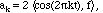
 t),
sin(4 t), ...,
sin(20 t),
cos(2 t),
cos(4 t), ...,
cos(20 t),
(f1)
t),
sin(4 t), ...,
sin(20 t),
cos(2 t),
cos(4 t), ...,
cos(20 t),
(f1)
Linear Methods of Applied Mathematics
Evans M. Harrell II and James V. Herod
version of 14 October 1997.
If you wish to print a nicely formatted version of this document, you may download the rtf file for Chapter II, which will be interpreted and opened by Microsoft Word. This document appears there as an appendix.
Some of the calculations of this chapter are available in a Maple worksheet or in a Mathematica notebook.
An intuitive way to understand projections of functions, which has many applications in signal processing, is in terms of filtering. The word "filtering" refers to an attempt to extract the important part of some data while eliminating random contributions called "noise" or other unwanted features which obscure the ones that matter. Electrical engineering offers many examples of filtering, which you are probably aware of as a consumer if you have a stereo system and a collection of recordings, but the notion is much more widely applicable than that.
To emphasize this, we call upon a less familiar example, drawn from astronomy. In recent years astonomomers have obtained reliable evidence that several nearby stars are orbited by planet-sized companions. The evidence was extracted from observations of the positions of the stars taken over periods of several years. How was this accomplished? As we all know, stars twinkle, which means that the image of the star moves in an erratic way at high frequencies, due to motions in our atmosphere. Other contributions to the motion of the image include the motion of the earth, which has daily, monthly, and yearly components, and human activities such as calibration, maintenance and cleaning of the facilities. Indeed, the first claimed proofs that a nearby star, Barnard's star, had an orbiting companion, were retracted when it became apparent that the periodic motion which was extracted from observations correlated with regularly scheduled human activities at the Swarthmore College Sproul Observatory ( image).
Many of these contributions are much larger than ones corresponding to planetary motion, and it is the task of the astronomer to filter out the unwanted contributions and see whether the remaining parts of the signal reveal a regular wobble, as would be caused by a planet.
Fortunately, this task is rather straightforward and can be reliably be solved with the tools of linear mathematics. All we need to do is use the same formula which allows us to project a vector onto another vector, in order to separate various contributions to a function.
To illustrate the procedure, we simplify the selection of features which are regarded as good or bad. Suppose that we have a signal f(t) which contains some pure frequencies we are interested in, say corresponding to pure vibratory functions
sin(2 t),
sin(4 t), ...,
sin(20 t),
cos(2 t),
cos(4 t), ...,
cos(20 t),
(f1)
with frequencies 1,2,..., 10, plus some noise fnoise(t). (The frequency of a
sinusoidal function sin( t) differs from the angular frequency
by the factor
2 .) We write the full function
in the form:
t) differs from the angular frequency
by the factor
2 .) We write the full function
in the form:
f(t) = a0 + a1 cos(2 t)
+ a2 cos(4 t)
+ ... a10 cos(20 t)
+ b1
sin(2 t) +
b2 sin(4 t)
+ ... b10
sin(20 t)
+ fnoise(t)
=: ffiltered(t) + fnoise(t)
Often the constant term a0 is left out of the expansion, since a signal usually oscillates around average zero.
A model problem in signal processing is to take a measured signal f(t) and extract from it the low frequency part while projecting away fnoise. The goal, then, is to determine the coefficients
a1, ..., a10 and b1, ..., b10.
As explained in Chapter II, the projection formula tells us the best choice for these coefficients, in the sense that the r.m.s. error
||fnoise(t)|| = ||f - (a1 cos(2
t) + ...+
b10 sin(20 t))||
is as small as possible, just as the projection of a vector into a plane is the planar vector whose distance from the original vector is as small as possible.
The projection formula for the orthogonal set (f1) on the basic period 0 < t < 1 tells us that
and similarly for the coefficients bk.
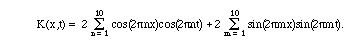
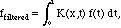
Notice that if we put these terms together, we see that the filtering is accomplished by an integral operator of the separable type,
We discuss the theory of such integral operators in a later chapter.
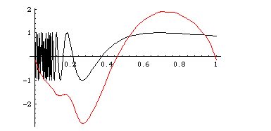
Example F.1 With the aid of mathematical software (see the Maple worksheet or Mathematica notebook), we can see the effect of filtering as applied to some interesting functions on the interval 0 < x < 1. Here we focus on the function sin(1/(x-.05)), which oscillates strongly near x=0 (graph). In the first calculation we filter out the frequencies greater than 3 - this would be called a low-pass filter - and compare with the unfiltered function on a common graph:
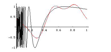
The match is rather good where the original function is varying slowly, but its high-frequency wiggles are filtered out.
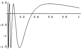
For comparison, let's look at the high-frequency part of the same function. A high-pass filter would throw away the result of the low-pass filter and keep the rest:
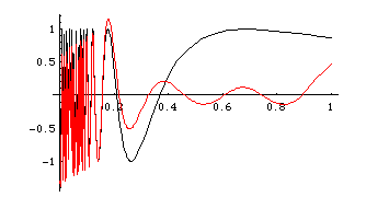
Here, the gently varying part of the function has been filtered out, and the wiggles remain.
Example F.2. If we modify the integral kernel K(x,t) as given above to

the result would be a signal which has its higher frequencies diminished in comparison with the lower ones (and has lost the frequencies above 10 altogether). Here is a plot (see the Maple worksheet or the Mathematica notebook) of the same function as used in Example F.1 along with the function obtained by signal processing with the kernel K:
Of course it matches less well than the low-pass filter of Example F.1: We have emphasized the low frequencies.