Linear Methods of Applied Mathematics

Evans M. Harrell II and James V. Herod*

*(c) Copyright 1994,1995,1996 by Evans M. Harrell II and James V. Herod. All rights reserved.

XIV. Ordinary differential operators

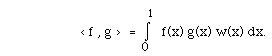
Recall that L²[0,1] is an inner product space when we provide it with the "usual" inner product. You should also recall there are many choices that can be made for an inner product for the functions on [0,1]. One might have a weighted inner product such as we had in Rⁿ and as was described in an appendix to Chapter II. That is, if w(x) is a continuous, non-negative function, we might have

The choices for w(x) are usually suggested by the context in which the space arises.

Some inner product spaces are called HILBERT SPACES. A Hilbert space is simply a vector space on which there is an inner product and on which there is one more bit of structure. A Hilbert space is a complete inner product space. This means that if f_p is an infinite sequence of vectors in the space which is Cauchy convergent - meaning that

lim_n,m < f_n-f_m , f_n-f_m > = lim_n,m | f_n-f_m |² = 0

- then there is a vector g, also in the space, such that lim_n f_n = g.

To illustrate these ideas, two examples follow. In the first, there is a sequence {f_p} and a function g in the space with

lim_n f_n = g. In the second, there is no such g.

EXAMPLE: Let E be the vector space of continuous functions on [0,1] with the usual inner product. Let

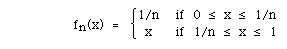
and let g(x) = x on [0,1]. Then lim_n |f_n - g|²

EXAMPLE. This space E of continuous functions on [0,1] with the "usual" inner product is not complete. To establish this, we provide a sequence f_p for which there is no continuous function g such that lim_n f_n = g.

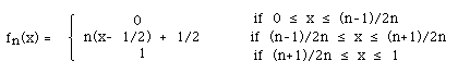
Sketch the graphs of f₁, f₂, and f₃ to see that the limit of this sequence of functions is not continuous.

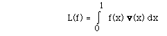
The Riesz Representation Theorem is an important idea in a Hilbert space. You will recall that in Rⁿ, this result declared that if L is a linear function from Rⁿ to R then there is a vector v in Rⁿ such that L(x) = < x, v > for each x in Rⁿ. (More description of the analogue of Riesz representation for Rⁿ.)

In general, where the vector space is not Rⁿ, more is required.

THEOREM If {E, < , >} is a Hilbert space, then these are equivalent:

(a) L is a continuous, linear function from E to R (or the complex numbers C), and

(b) there is a member v of E such that L(x) = < x, v > for each x in E.

It is not hard to show that (b) implies (a). To show that (a) implies (b) is more interesting. The argument uses the fact that E is complete and can be found in any introduction to Hilbert space or functional analysis.

EXAMPLE. Since the space of continuous functions on [0,1], denoted C[O,1], with the usual inner product is not a Hilbert space, one should expect that there might be a linear function L from C[0,1] to R for which there is no v in C[0,1] such that

for each f in C[0,1]. In fact, here is such an L:

Let

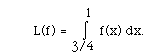
The candidate for v is v(x) =1 on [3/4, 1] and 0 on [0, 3/4). But this v is not continuous! It is only piecewise continuous.

DEFINITION. The Heaviside function H is defined as follows:

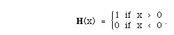
                                                                                                                 (14.1)

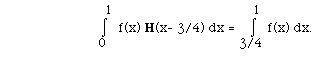
Thus, the Heaviside function provides an element v for which the linear function

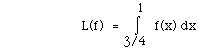
has a Riesz representation. As noted, v is not in C[0,1].

It is not always possible to have a piecewise continuous v which will rectify the situation. Consider the following linear function: L(f) = f(1/2). It is not so hard to see that there is no piecewise continuous function v on [0,1] having the property that for every continuous f,

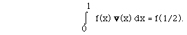
DEFINITION. The symbol \delta is used to denote the "generalized" function which has the property that

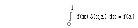
                                                                                                                 (14.2)

for some suitably large class of functions f, when 0 < a < 1. It is no surprise that some effort has been made to develop a theory of generalized functions in which the delta function can be found. Generalized functions are also called "distributions". While the delta function is not a well-defined function of the familiar type, it can be manipulated like a function in most cases, provided that in the end it will be integrated, and that the other quantities in the integral with it will be continuous.

A suggestive analogy is that of complex numbers. Like complex numbers, generalized functions are idealizations which do not describe real, physical things, but they have been found tremendously useful in applied mathematics. Most famously they were used by Dirac in his quantum mechanics; it is less well known that mathematical physicist Kirchhoff used them decades earlier in his work on optics. The theory of distributions is attractive and establishes a precise basis for the ideas which these notes will use. It is the choice of this course and these notes, however, to use the delta function without exploring the mathematical framework in which it should be studied.

We shall return to the delta function when its properties are needed to understand how to construct Green functions.

As suggested in the first two chapters the role of the adjoint of a linear function will be critical. If L is a linear function that is defined on some subspace of E, then the task of finding the adjoint L* will involve finding not only how the adjoint is defined, but also what is the subspace composing the domain of L*.

Consider the differential operator L given by

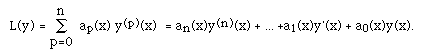
One often defines the formal adjoint L* of L by

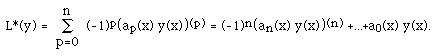
                                                                                                                 (14.3)

The second order operator L(y) = a₂(x) y''(x) + a₁(x) y'(x) + a₀(x) y(x), according to this formula, will have formal adjoint

L*(y) = (a₂(x) y(x))'' - (a₁(x) y(x))' + a₀(x) y(x).

If L is not defined on all of E, but just some subspace, or manifold M, then one must find where L* is defined. We denote the domain of L* by M*.

DEFINITION. Suppose that L is defined on a manifold, or subspace, M, and that L* is defined on a manifold M*. Then L* is THE adjoint of L if

                                                                                                                 (14.4)

for all u in M and v in M*.

EXAMPLE Let L(u) = u''(x) + 3x u'(x) + x² u(x) be defined on the manifold consisting of all functions u on [0,1] which satisfy u(0) = u'(1) and u(1) = u'(0),

M = {u:u(0) = u'(1), u(1) = u'(0)}.

We indicated how to find L* and M*.

L*(v) = v'' - (3x v(x))' + x²v(x).

The manifold M* is chosen to make the equation

< L(u), v> = < u, L*(v) >

satisfied.

Since u is in M, u'(1) = u(0) and u(1) = u'(0), so that

< L(u), v > - < u, L*(v) > = [v(1) + v'(0)]u(0) - v'(1) + v(0) - 3v(1)] u'(0).

In order for this last line to be zero for all u in M, the manifold M* should consist of functions f such that

v(1) + v'(0) = 0 and v'(1) + v(0) = 3v(1).

                                                                                   QED

TYPICAL PROBLEM:

The problem y''+ 3y' + 2y = f , y(0) = y'(0) = 0 leads to an operator L and a manifold M given by

L(y) = y'' + 3y'+2y and M = {y: y(0) = y'(0) = 0 }.

The problem is to solve the following equation: given a continuous function f, find y in M such that L(y) = f. The technique is to construct a function G such that u is given by

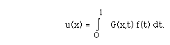
For such problems, we will have techniques to construct G. In this case

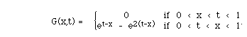
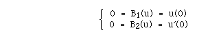
Most frequently, we will consider three types of boundary conditions illustrated below for a second order problem:

Initial conditions

unmixed, two point boundary conditions

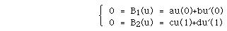
mixed, two point boundary conditions

Before developing a technique for solving these ordinary differential equations with boundary conditions, attention should be paid to the statement of the Fredholm Alternative Theorems in this setting. You may wish to compare it with the alternative theorems for integral equations and for matrices.

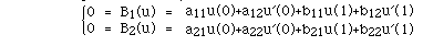
Suppose that L is an n^th order differentiable operator with n boundary conditions. B₁, B₂, ...B_n. The problem is posed as follows: Given f, find u such that L(u) = f with B_p(u) = 0, p = 1, 2, ...n.

I. Exactly one of the following two alternatives holds:

(a)(First Alternative) if f is continuous then L(u) = f, B_p(u) = 0, p = 1, 2, ..., n, has one and only one solution..

(b)(Second Alternative) L(u) = 0, B_p(u) = 0, p = 1, 2, ...n, has a nontrivial solution.

II. (a) If L(u) = f, B_p(u) = 0, p = 1, 2, ...n, has exactly one solution then so does L*(u) = f, B_p*(u) = 0, p = 1, 2, ...n have exactly one solution.

(b) L(u) = 0, B_p(u) = 0, p = 1, 2, ... n, has the same number of linearly independent solutions as L*(u) = 0, B_p*(u) = 0, p = 1, 2, ...n.

III. Suppose the second alternative holds. Then L(u) = f, B_p(u) = 0, p = 1, 2, ...n has a solution if and only if < f, w > = 0 for each w that is a solution for
   L*(w) = 0, B_p*(w) = 0, p = 1, 2, ...n.

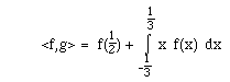
XIV.2.   Let <f,g> denote the standard inner product for 0 <= x <= 1.

Find a generalized function g(x) such that

XIV.3.   Compute the formal adjoint for each of the following:

(a) L(y) = x² y'' + x y' + y (b) L(y) = y'' + 9 \pi² y

(c) L(y) = (e^x y'(x))' + 7 y(x) (d) L(y) = y'' + 3y' + 2y

XIV.4.   Argue that L is formally self adjoint if it has constant coefficients and derivatives of even order only.

XIV.5.   Suppose that L(y) = y'' + 3y' + 2y and y(0)= y'(0) = 0.

Find conditions on v which assure that

XIV.6.   Let L(u) = u'' + u. The formal adjoint of L is given by L*(v) = v''+ v. For each manifold M given below, find M* such that L* on M* is the adjoint of L on M.

(a) M = {u: u(0)=u(1)=0},

(b) M = {u: u(0)=u'(0)=0}

(c) M = {u: u(0)+3u'(0)=0, u(1)-5u'(1)=0},

(d) M = {u: u(0)=u(1), u'(0)=u'(1) }.

       (Answers)

XIV.7.   Let L and M be as given below; find L* and M*.

(a) L(u)(x) = u''(x) + b(x) u'(x) + c(x) u(x),

M = {u: u(0)=u'(1), u(1) = u'(0) }.

(b) L(u)(x) = -(p(x) u'(x))' + q(x) u(x);

M = {u: u(0) = u(1), u'(0) =u'(1) }.

       (Hint) (c) L(u)(x) = u''(x);

M = {u: u(0) + u(1) = 0, u'(0) - u'(1) = 0 }

       (Answers)

XIV.8.   Verify that for L, M, and u as given in the TYPICAL PROBLEM above, u is in M and L(u) = f. (Recall Exercise 3 in the introduction to the problems of Green functions.)

Suppose G is as in the TYPICAL PROBLEM and

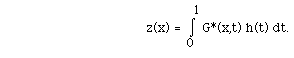
Show z solves L* on M*.

XIV.9.   Decide whether the following operators L are formally self adjoint, and whether they are self adjoint on M. Decide whether the equation L(y) = f on M is in the first or second alternative.

(a) L(y) = y'', M = {y: y(0) = y'(0) = 0 }.
       (Answer)

(b) L(y) = y'', M= {y: y(0) = y(1) = 0 }.
       (Answer)

(c) L(y) = y'' + 4 \pi ²y, M={y: y(0) = y(1), y'(0) = y'(1)}.
       (Answer)

(d) L(y) = y'' + 3y' + 2y, M = {y: y(0) = y(1) = 0}.
       (Answer)

XIV.10.   Suppose that L(y)(x) = y''(x) + 4 \pi ²y(x). B₁(y) = y(0) and B₂(y) = y(1).

(a) Show that the problem L(y) = 0, B₁(y)= B₂(y) = 0 has sin(2 \pi x) as a non-trivial solution.

(b) What is the adjoint problem for {L, B₁, B₂}?

(c) What specific conditions must be satisfied by f in order that L(y) = f, y(0) = 0 = y(1) has a solution?

(d) Show that y''(x) + 4 \pi ²y(x) = 1, y(0) = 0 = y(1) has

[ 1 - cos(2 \pi x) ] /4 \pi ² as a solution.

XIV.11.   Show that y'' = x, y'(0) = 0 = y'(1) has no solution.

XIV.12.   Show that y'' = sin(2 \pi x), y'(0) = 0 = y'(1) has a solution.

Onward to Chapter XV

Back to Chapter 13 (beginning) (second part)

Return to Table of Contents

Return to Evans Harrell's home page